Historical Context

This review lands at a pivotal moment in computational biology — 2017, right at the cusp between the "coevolution era" and the "deep learning era" of protein structure prediction. It synthesizes a decade of work using statistical physics to understand protein sequences.

The Lineage

1. Early 2000s: People noticed that mutations at two positions in a protein family tend to be correlated if those residues are in physical contact. Simple covariance matrices from MSAs could hint at contacts, but they were noisy — indirect correlations muddied everything.
2. 2009–2011 — Direct Coupling Analysis (DCA): Weigt et al. (2009) and Morcos et al. (2011) borrowed from statistical physics — specifically spin-glass models — and applied the maximum entropy principle: find the simplest probability distribution over sequences that reproduces the observed single-site and pairwise frequencies from the MSA. This gives you a Potts Hamiltonian. The coupling parameters directly separate real contacts from transitive noise. Contact prediction accuracy jumped dramatically.
3. 2013 — Pseudolikelihood methods (PLM): Kamisetty, Ovchinnikov & Baker showed that pseudolikelihood maximization was faster and more accurate for contact prediction than mean-field DCA. This became the workhorse method.
4. 2014–2016 — Beyond contacts: People realized the Potts model isn't just a contact predictor — it's a statistical model of the entire sequence landscape. The Hamiltonian H(S) correlates with folding free energy ΔG, with fitness, and can capture epistasis.

A Gentle Introduction to Hamiltonian Models for Protein Sequences

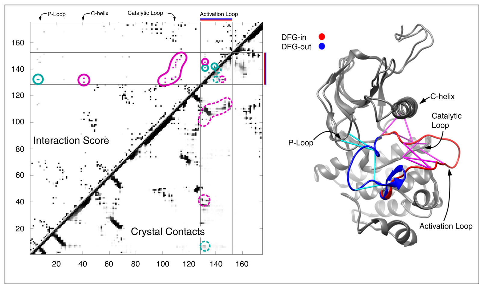
The basic question: Given a family of related protein sequences (say, thousands of kinase sequences from across the tree of life), can we build a mathematical model that captures why certain amino acid combinations appear together and others don't?

Start with the simplest model — independent sites. Imagine each position in the protein evolves independently. Position 42 "likes" to be leucine 60% of the time, valine 30%, etc. This is essentially a Position-Specific Scoring Matrix (PSSM). It works okay for sequence search, but it misses something huge: correlations between positions.

The Hamiltonian — an energy function over sequences. Borrowing from statistical physics, we assign every possible sequence S a statistical score:

The Fields: h_i(s_i)

The site-wise bias — how much position i "prefers" each of the 21 possible amino acids (20 + gap), independent of everything else. It captures the frequency of each amino acid at this position across all sequences in the MSA.

If position 50 is always glycine (say, because it's in a tight loop where only glycine fits sterically), then h₅₀(Gly) will be very favorable and h₅₀(Trp) very unfavorable. If a position is highly variable, the fields will be relatively flat.

This component is equivalent to a PSSM. If you only had the fields and no couplings, you'd have an independent model — each position does its own thing.

The Couplings: J_ij(s_i, s_j)

This is where the power is. J_ij(s_i, s_j) asks: given that position i is amino acid A and position j is amino acid B, is that combination more or less likely than you'd expect from the individual frequencies alone?

It's not a single number per pair — it's a 21×21 matrix for every pair (i,j). So J₁₂(Lys, Glu) might be very favorable because a salt bridge forms, while J₁₂(Lys, Lys) might be unfavorable because you've got two positive charges clashing.

The critical insight of DCA is that raw correlations in the MSA mix direct and indirect effects. If residue A contacts B, and B contacts C, then A and C will look correlated even if they never interact. The Potts model inversion disentangles this — the J parameters represent direct couplings.

Scale

For a 100-residue protein, the full Hamiltonian has:

• 100 × 21 = 2,100 field parameters
• C(100,2) × 21 × 21 ≈ 2.2 million coupling parameters

That's a lot of parameters, which is why you need deep MSAs (thousands of sequences) to fit the model. It's also why this approach struggled for orphan proteins with few homologs — a limitation that protein language models like ESM later solved by sharing information across families.

The Intuition

The Probability of a Sequence

Follows the Boltzmann distribution: P(S) ∝ exp(−H(S)). Sequences with low H(S) are common in the family. Sequences with high H(S) are rare or nonexistent. This is the maximum entropy model — the least biased distribution that reproduces observed frequencies.

Important caveat: H(S) is a statistical score, not a physical energy in kilocalories. The fact that it correlates with physical ΔG is an empirical observation, not a derivation. It's a statistical look-up table, not an energy landscape.

The Potts → Evoformer Connection

The architectural parallel between the Potts model and AlphaFold2's Evoformer is striking and almost certainly not coincidental:

Potts Model	Evoformer (AlphaFold2)
hi(si) — fields per position	MSA representation — per-residue embeddings via row/column attention
Jij(si, sj) — 21×21 coupling matrix per pair	Pair representation — full L×L matrix of pairwise embeddings
Inverse inference from MSA frequencies	Learned end-to-end from MSA + structure supervision
Maximum entropy (least biased fit)	Transformer (massively overparameterized, regularized by data)

The Evoformer's MSA track processes rows (individual sequences) and columns (positions across sequences). The column attention reads off single-site statistics analogous to h_i. The row attention lets sequences talk to each other — extracting covariation patterns.

The pair track maintains an explicit L×L matrix updated by outer products from the MSA track. This is the coupling matrix, except instead of 21×21 scalars, it's a rich learned embedding. The triangular attention enforces geometric consistency — exactly the transitivity correction DCA performs when separating direct from indirect couplings.

The Historical Thread

Potts/DCA (2009–2013) → coevolution contacts + Rosetta (Baker lab, 2015–2017) → trRosetta (2020) → AlphaFold2 Evoformer (2021). The two-track decomposition (single-site + pairwise) was inherited from decades of coevolutionary analysis. Deep learning replaced the statistical physics inference with a neural network that could learn far richer representations.

Epistasis — Context-Dependent Mutation Effects

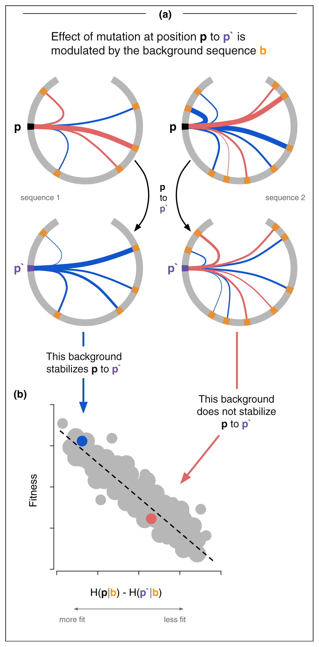
Definition: Epistasis is when the effect of a mutation depends on what other mutations are already present in the sequence. A mutation that's deleterious in one background can be neutral or even beneficial in another. The whole is not the sum of the parts.

In Potts model terms, epistasis is literally encoded in the couplings J_ij(s_i, s_j). If you mutate position i, the fitness effect depends on what's at every coupled position j. This is why the independent model (fields only, no couplings) systematically underperforms.

This term deserves more use in the protein ML field — when people talk about "context-dependent mutation effects" or "non-additive interactions," they're describing epistasis.

The Numbers: Potts ΔH vs. Experimental Fitness

Study	System	Correlation	Notes
Figliuzzi et al. 2015	TEM-1 beta-lactamase (DMS)	R = 0.74 (R² = 0.55)	ΔH vs. ΔΔG: R = 0.81. Independent model only R = 0.63
Ferguson et al. 2013	HIV-1 Gag (replicative fitness)	ρ = −0.81	50 engineered mutants. Regularized: r = −0.85, AUROC = 0.93
Hopf et al. 2017 (EVmutation)	34 DMS datasets	ρ = 0.4–0.87	Best: beta-lactamase 0.87, HIV 0.81. ProteinGym avg: 0.397
Barton et al. 2016	HIV immune escape timing	r = 0.66–0.81	86% correct escape location. Entropy alone: pseudo-R² = 0.05

Inference Methods

The method used to infer Potts parameters changes the answer, not just the speed:

Method	Speed	Accuracy	Best for
Mean-field DCA	Very fast	Approximate	Contact prediction
Pseudolikelihood (PLM)	Fast	Good	Contact prediction
Monte Carlo	Slow	Exact	Fitness/energy prediction
ACE (Adaptive Cluster Expansion)	Moderate	Good	Fitness/energy prediction

Mean-field DCA underestimates sequence diversity and generates overly fit sequences. PLM tends to produce less stable sequences than reality. Only Monte Carlo and ACE faithfully reproduce the actual MSA statistics.

What a Simple Reading Might Miss

1. The phylogenetic correction is hand-waved. The Potts model assumes each MSA sequence is an independent draw from P(S). That's wrong — sequences are related by a phylogenetic tree. The fix (cluster at ~80% identity, reweight) is crude. Every correlation number has an asterisk.
2. No insertions or deletions. The Hamiltonian is defined over a fixed-length aligned sequence. Gaps are a 21st character, which is a hack. The model fundamentally can't reason about indels — a limitation protein language models later solved.
3. 2.2 million parameters need deep MSAs. For shallow MSAs (orphan proteins, designed proteins), the model fails. This is exactly the gap ESM was built to fill, and why the ProteinGym average drops to ρ ≈ 0.4.
4. The "energy" is not energy. H(S) is a statistical score. The correlation with ΔG is empirical, not derived. The bridge (evolutionary selection pressure) assumes near-neutral evolution and folding stability as the dominant fitness determinant, which don't always hold.
5. HIV fitness validation has selection bias. The model trains on in vivo sequences but validates against in vitro fitness. The engineered mutants were chosen to span a predictable range, not sampled randomly.
6. The Potts model is already a generative model. You can sample from P(S) via MCMC. This was done in some referenced work but wasn't the focus. In hindsight, this is the direct precursor to modern generative protein design — the leap from "score sequences" to "sample new ones" was there in 2017.

Bottom Line

This paper is the intellectual ancestor of the modern protein ML stack. The Potts Hamiltonian — a statistical look-up table built from sequence co-variation, decomposed into per-site fields and pairwise couplings — achieves remarkable predictive power for fitness, stability, and structural contacts. Its two-track decomposition (single-site + pairwise) directly prefigures the Evoformer architecture. Its limitations (deep MSA requirement, fixed-length, no geometry) are exactly the problems that protein language models and structure prediction networks were built to overcome.

This is the baseline that every protein ML model is implicitly competing against.

Key References Discussed

1. Weigt M, White RA, Szurmant H, Hoch JA, Hwa T. Identification of direct residue contacts in protein–protein interaction by message passing. PNAS 106:67–72, 2009. doi:10.1073/pnas.0805923106 — Introduced Direct Coupling Analysis (DCA) using message passing.
2. Morcos F et al. Direct-coupling analysis of residue coevolution captures native contacts across many protein families. PNAS 108:E1293–E1301, 2011. doi:10.1073/pnas.1111471108 — Scaled DCA to many protein families using mean-field approximation.
3. Kamisetty H, Ovchinnikov S, Baker D. Assessing the utility of coevolution-based residue–residue contact predictions in a sequence- and structure-rich era. PNAS, 2013. doi:10.1073/pnas.1314045110 — Showed pseudolikelihood (PLM) outperforms mean-field DCA for contact prediction. A direct stepping stone to trRosetta and AlphaFold2.
4. Ferguson AL et al. Translating HIV sequences into quantitative fitness landscapes predicts viral vulnerabilities for rational immunogen design. Immunity 38:606–617, 2013. doi:10.1016/j.immuni.2012.11.022 — Demonstrated ρ = −0.81 correlation between Ising model energy and HIV-1 Gag replicative fitness across 50 mutants.
5. Figliuzzi M et al. Coevolutionary landscape inference and the context-dependence of mutations in beta-lactamase TEM-1. Mol Biol Evol 33:268–280, 2016. doi:10.1093/molbev/msv211 — Potts ΔH vs. DMS fitness: R = 0.74; vs. ΔΔG: R = 0.81. Independent model only R = 0.63.
6. Barton JP et al. Relative rate and location of intra-host HIV evolution to evade cellular immunity are predictable. Nat Commun 7:11660, 2016. doi:10.1038/ncomms11660 — Potts + Wright-Fisher predicts immune escape timing (r = 0.66–0.81) and location (86% correct). Entropy alone: pseudo-R² = 0.05.
7. Hopf TA et al. Mutation effects predicted from sequence co-variation. Nat Biotechnol 35:128–135, 2017. doi:10.1038/nbt.3769 — EVmutation: Potts model across 34 DMS datasets, ρ = 0.4–0.87. Disease variant AUC = 0.89–0.96.
8. Jumper J et al. Highly accurate protein structure prediction with AlphaFold. Nature 596:583–589, 2021. doi:10.1038/s41586-021-03819-2 — Evoformer architecture inherits the two-track (single-site + pairwise) decomposition from coevolutionary analysis.