Teaching a Protein Language Model to Speak "Immune"

Here's a fact that keeps immunologists up at night: your immune system has to figure out which tiny protein fragments (peptides) sitting on the surface of your cells are "self" versus "intruder." This recognition happens through a molecular handshake between peptides and MHC class I molecules — and it's the foundation of how your body fights cancer. If we could predict which peptides bind well to which MHC molecules, we could design better cancer vaccines and T-cell therapies. The problem? There are roughly 30,000 known HLA alleles (the human version of MHC), and for most of them, we have almost no experimental binding data.

This is the problem that led me, along with Ariel and Nilah, to ask a deceptively simple question: can we take an off-the-shelf protein language model — one that already "understands" proteins in general — and teach it to specialize in the language of immune recognition?

The Intuition: Language Models Already Know Proteins

Large protein language models like ESM Cambrian have been trained on millions of protein sequences. They've learned a kind of grammar — which amino acids tend to appear together, what patterns form functional domains, how evolution shapes sequence diversity. Think of it like a model that's read every book ever written. It understands English really well. But if you need it to write radiology reports, it would help to let it read a bunch of medical literature first, right?

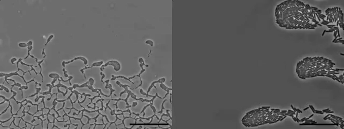
That's exactly what continued pre-training is. We took ESM Cambrian (300 million parameters, 30 transformer layers) and gave it a reading list of HLA-associated peptides from the IEDB — the main repository of immune epitope data. The model didn't get any labels at this stage. It just learned to fill in masked amino acids in peptide sequences, the same masked-language-modeling trick that made BERT famous. The idea is that by seeing thousands of peptides in the context of their MHC partners, the model would internalize the subtle patterns of what makes a peptide "MHC-compatible."

The Key Insight: When Does This Actually Help?

Here's what surprised us. The benefit of continued pre-training wasn't universal — it depended on how much labeled data you had for a given allele. We found a clear sweet spot:

For alleles with very few measurements (under 500 peptides), the continued pre-training didn't help much. The model simply didn't have enough downstream examples to leverage its new knowledge. For alleles with moderate data (500 to 2,000 peptides), continued pre-training gave us a boost of about 0.10 in Spearman correlation — a meaningful jump in this field. And for data-rich alleles (over 4,000 peptides), the gains leveled off because there was already enough signal in the fine-tuning data.

That moderate-data regime is exactly where most clinically relevant alleles live. So the technique lands where it matters most.

A Deliberate Choice: No Mass Spec

One decision we were pretty deliberate about was training exclusively on IC50 binding affinity data from functional assays and completely avoiding mass spectrometry data. Mass spec datasets are huge and tempting, but they systematically over-represent peptides with canonical anchor residues. They tell you what was easy to detect, not necessarily what binds. By sticking to quantitative IC50 measurements — log-transformed and rebalanced — we traded quantity for quality. And it paid off.

How Did We Do?

When we benchmarked against state-of-the-art tools on a held-out test set of peptides deposited in IEDB between 2020 and 2025, our model (ESMCBA) achieved a median Spearman correlation of 0.62 across 25 common HLA alleles. For comparison, NetMHCpan 4.1 — the field's workhorse, an ensemble of 50 networks trained on over 13 million data points — scored 0.56. MHCflurry came in at 0.49. We also outperformed NetMHCpan on distinguishing low-affinity binders from intermediate-affinity binders (AUROC 0.95 vs. 0.84), which is arguably the classification that matters most for therapeutic peptide selection.

Not bad for a single model with some targeted reading.

So What Does This Mean?

The broader takeaway is pretty encouraging: you don't always need a massive domain-specific dataset or a bespoke architecture. Sometimes, modest and targeted continued pre-training on a strong foundation model can get you surprisingly far. Going forward, we're excited about extending this to MHC class II, incorporating structural features, and exploring whether these adapted representations can help with the even harder problem of predicting immunogenicity — not just whether a peptide binds, but whether it actually triggers a T-cell response. That's where the real clinical impact lives.

This work was accepted at the 20th Machine Learning in Computational Biology (MLCB) meeting.

What If We Could Design Immune Peptides from Scratch — Using Physics Instead of Data?

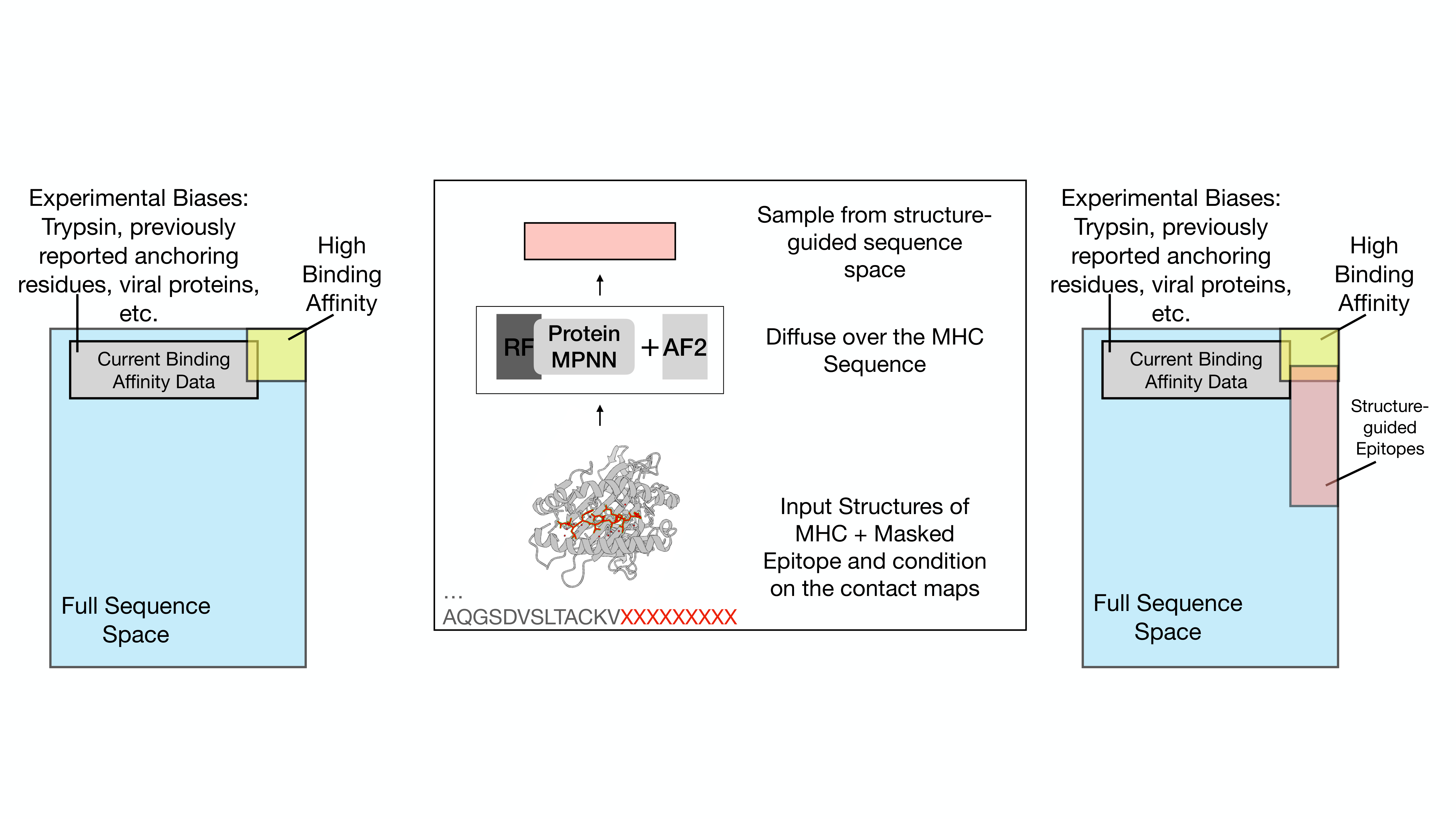
If you've been following the MHC binding prediction space, you've probably noticed a pattern: everyone trains on the same datasets, benchmarks on the same test splits, and reports incremental improvements. But there's an uncomfortable question lurking underneath all of this — what if those datasets are biased in ways that make our models look better than they actually are?

That question is what drove this project. Together with Ariel and Nilah, we set out to build a benchmark of MHC-binding peptides that doesn't come from the usual experimental pipelines. Instead, we designed peptides from scratch using diffusion models conditioned on crystal structure geometry. The goal was to create peptides that should bind — based on physical structure — but that no existing model has ever seen during training.

The Problem with Current Benchmarks

Most of the peptide-MHC data we have comes from mass spectrometry experiments or binding assays. These methods are fantastic, but they have blind spots. Mass spec systematically under-detects certain peptides (cysteine-containing ones, for instance) and over-represents peptides with strong canonical anchor residues. When you train a model on biased data, you get a model that's great at recognizing the patterns in that bias — and not necessarily great at recognizing genuine binding.

It's like training a food critic exclusively on Italian restaurants and then asking them to evaluate Thai food. They might still have good instincts, but you wouldn't fully trust the score.

Our Approach: Let the Structure Do the Talking

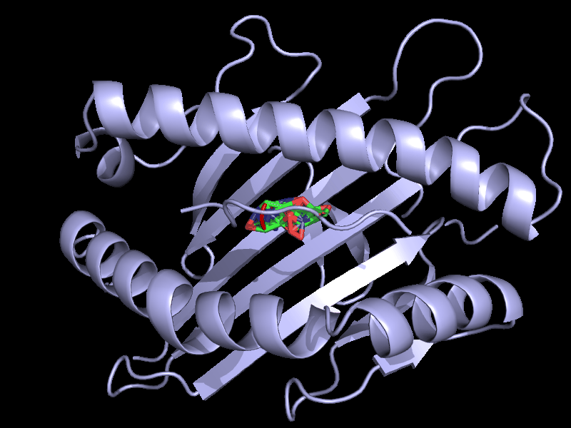
Here's the idea. We have about 119 high-resolution crystal structures of peptide-MHC complexes sitting in the Protein Data Bank. These structures show us, at atomic resolution, exactly how peptides nestle into the MHC binding groove — which residues make close contacts (within 3.5 angstroms), which ones form looser associations (3.5 to 5.0 angstroms), and where the anchoring happens.

We used these contact maps as conditioning constraints for RFdiffusion, a structure-generation diffusion model. The process works like this: we take an MHC crystal structure, rip out the peptide, and ask RFdiffusion to hallucinate a new peptide backbone that fits the groove. We run 50 diffusion steps, generating backbones for peptides of 9 to 11 residues. Then we hand those backbones to ProteinMPNN, which designs 64 amino acid sequences per backbone and ranks them by fit. Finally, we fold every designed peptide-MHC complex with AlphaFold2-Multimer and filter for structural confidence — keeping only designs where the peptide pLDDT hits at least 0.80.

The result is a library of computationally designed peptides spanning 27 HLA alleles that should be structurally compatible with their MHC partners, but that were never derived from any experimental binding dataset.

The Fun Part: Breaking Existing Predictors

This is where things got really interesting. We took seven state-of-the-art binding predictors — NetMHCpan, MHCflurry, HLApollo, HLAthena, MixMHCpred, MHCnuggets, and our own ESMCBA — and asked them to distinguish our structurally designed peptides from experimentally validated strong binders. If these predictors truly understand MHC binding, they should score our well-designed peptides similarly to known binders.

They didn't. AUROCs ranged from 0.03 (MHCnuggets) to 0.19 (HLApollo). That's essentially random or worse. The same predictors scored above 0.88 when discriminating validated binders from random peptides — so they're not broken in general. They just can't recognize binding potential in peptides that look different from their training data.

This is a big deal. It means there are entire regions of peptide sequence space that are structurally plausible binders but invisible to current tools.

Sanity Check: Do the Designs Make Biological Sense?

We were careful to check that our diffusion pipeline wasn't just generating nonsense. When we looked at anchor residue preferences, the designs reproduced known biology beautifully. For HLA-A*02:01, we saw the expected Leucine enrichment at position 2 and Valine at the C-terminus. For HLA-B*57:01, the signature Tryptophan anchor at the C-terminus showed up clearly. And peptides with proper anchors had significantly higher AlphaFold2 confidence scores — so the structural validation and the sequence motifs aligned perfectly.

Why This Matters

We see this resource serving two purposes. First, it's an unbiased benchmark. If you're developing a new binding predictor, you can test it against these structurally designed peptides to see whether it's truly learning binding physics or just memorizing dataset patterns. Second, these libraries represent a starting point for discovering genuinely novel peptide ligands — candidates that existing methods would overlook but that might make excellent vaccine targets or therapeutic leads.

Next, we want to incorporate T-cell receptor constraints into the design pipeline — because binding to MHC is only half the story. The peptide also has to be recognized by a T-cell receptor to trigger an immune response. That's the real frontier.

This work was accepted at the 2nd Workshop on Generative AI and Biology at ICML 2025.

Protein Diffusion Models as Statistical Potentials

James P. Roney, Chenxi Ou, Sergey Ovchinnikov · bioRxiv, 2025

Alright, so here's the setup. Diffusion models have been crushing it in protein structure generation — you've probably heard of RFdiffusion and friends. But this paper asks a really clever question: what if instead of just using these models to generate new proteins, we could use them as energy functions? Like, what if the model's learned score function could tell us how "good" a given protein conformation is?

That's basically what ProteinEBM is. They take a pre-trained protein diffusion model and derive an energy-based model from it. The key insight is that the denoising process in a diffusion model implicitly learns a probability distribution over protein structures. If you can extract the energy landscape from that distribution, you've got yourself a statistical potential that knows what realistic protein conformations look like.

What's cool is how broadly useful this turns out to be. They show that ProteinEBM can rank the correctness of protein structures (which fold is more native-like?), do actual structure prediction from sequence, sample multiple conformational states of flexible proteins, and even predict the energetic effects of point mutations. And it's competitive with or better than both traditional physics-based force fields and other ML methods across these tasks.

The mutation effect prediction part is particularly interesting to me. There's been a ton of work on predicting delta-delta-G from sequence-based models, but having a structure-aware energy function that can do this feels like the right approach. You're literally asking "how does this mutation change the energy landscape?" which is what's actually happening physically.

The big picture here is that generative models contain way more information than we typically extract from them. We train them to generate, but the learned distribution itself is a rich model of protein physics. This paper is a nice reminder that sometimes the most interesting applications of a model aren't the ones it was originally trained for.

Read the paper

Designing Novel Solenoid Proteins with In Silico Evolution

Daniella Pretorius, Georgi I. Nikov, Kono Washio, Steve-William Florent, Henry N. Taunt, Sergey Ovchinnikov, James W. Murray · Communications Chemistry (Nature), 2025

Solenoid proteins are one of those protein architectures that feel almost too elegant. They're built from repeating structural units — think of them like a spiral staircase made of protein. Nature uses them everywhere: from beta-helices in antifreeze proteins to TPR repeats that mediate protein-protein interactions. But the natural repertoire of solenoid topologies is limited. What if we could design new ones?

This paper takes a really fun approach. Instead of using the fancy generative models that everyone's been working on lately, they go old school: a genetic algorithm. But with a twist — they use AlphaFold2 as the fitness function. So you have a population of sequences that evolve over generations, and at each step, AlphaFold2 tells them which sequences fold into the desired solenoid topology. There's also a solenoid discrimination network that helps filter candidates.

What I like about this is the simplicity of the concept. You don't need to train a specialized generative model. You just need a good oracle (AlphaFold2) and a search strategy (the genetic algorithm). It's kind of like directed evolution, but entirely in silico. And it works — they designed alpha-solenoids, beta-solenoids, and alpha-beta solenoids, spanning both natural topologies and folds that haven't been seen in nature.

The experimental validation is solid too. They picked a handful of designs, expressed them in E. coli, and got five that were highly stable. That's a 20% experimental success rate, which is actually pretty good for de novo protein design. It's not 100%, but for a method that's essentially guessing-and-checking with AlphaFold2, it's encouraging.

One thing that struck me is how this approach reveals that the space of possible solenoid topologies is larger than what nature has explored. There are stable folds out there that evolution just never stumbled upon. That's a pretty cool thought — we're not just redesigning nature, we're expanding the protein universe.

Read the paper

CIRPIN: Learning Circular Permutation-Invariant Representations

Aiden R. Kolodziej, S. Mazdak Abulnaga, Sergey Ovchinnikov · bioRxiv, 2025

Here's a problem that's been hiding in plain sight for years. Say you have two proteins that fold into essentially the same 3D shape, but one of them has its chain "rewired" — the N-terminus of one lines up with some internal position of the other. This is called circular permutation, and it's surprisingly common in nature. Proteins can evolve to swap where their chain starts and ends while keeping the same overall fold.

The problem? Most of our structural comparison tools — things like TM-align, Foldseek, DALI — are sensitive to chain topology. They compare structures in a way that cares about which residue comes first, second, third in the linear sequence. So two circularly permuted proteins that look basically identical in 3D can score as completely unrelated. That's a pretty big blind spot.

CIRPIN tackles this head-on with a graph neural network that's explicitly designed to be invariant to circular permutations. The clever bit is the data augmentation: during training, they synthetically circularly permute proteins so the model learns representations that are the same regardless of where you cut the chain. It's one of those ideas that seems obvious in hindsight but actually requires careful implementation.

The results are striking. They search through the SCOPe database and the AlphaFold Cluster Representatives and find thousands of novel circularly permuted pairs that previous methods completely missed. My favorite finding is that PDZ domains — one of the most studied protein families in structural biology — naturally exist in four distinct circularly permuted forms. Four! And we didn't know about some of these until CIRPIN found them.

This matters because circular permutation isn't just a structural curiosity. It can change a protein's function, stability, and interactions. If our homology detection tools are systematically missing these relationships, we're leaving a lot of biology on the table. CIRPIN fills that gap nicely.

Read the paper

Hit or Miss: Understanding Emergence and Absence of Homo-oligomeric Contacts in Protein Language Models

Zhidian Zhang, Yo Akiyama, Yehlin Cho, Samarth Jajoo, Sergey Ovchinnikov · bioRxiv, 2025

This one scratches a theoretical itch I've had for a while. Protein language models like ESM-2 are trained on individual protein sequences — single chains, one at a time. They never see protein complexes during training. And yet, when you extract attention maps or contact predictions from these models, they somehow know about inter-subunit contacts in homo-oligomers (proteins that assemble into copies of themselves). How?

The authors dig into this with a really systematic analysis. First, the scaling behavior is fascinating: as you make the model bigger, its ability to predict inter-chain contacts keeps improving, even after single-chain contact prediction accuracy has plateaued. That's a striking emergent property — the model discovers quaternary structure information as a byproduct of learning more about individual sequences.

There's also a cool comparison between ESM-2 and MSA-based approaches (MSA Pairformer). When you restrict multiple sequence alignments to close evolutionary neighbors, the MSA approach edges out ESM-2 on interface contact recovery (0.44 vs 0.33). But ESM-2 doesn't need any alignment at all — it works from a single sequence. So there's a tradeoff between the coevolutionary signal you get from alignments and the implicit knowledge baked into a massive language model.

One really practical result: the largest ESM-2 model can accurately distinguish genuine biological interfaces from crystal packing artifacts. This is a classic problem in structural biology — when you solve a crystal structure, you see contacts between protein copies in the crystal lattice, and it's not always obvious which of those contacts are biologically real. Having a sequence-based model that can make this call is genuinely useful.

The "hit or miss" framing in the title is apt. The model doesn't learn all interfaces equally. Some it nails, others it completely misses. Understanding which ones and why is where the real mechanistic insight lies, and this paper makes good progress on that front.

Read the paper

Assessing the Utility of Coevolution-Based Contact Predictions

Hetunandan Kamisetty, Sergey Ovchinnikov, David Baker · PNAS, 2013

Going back to 2013 for this one, and honestly, reading it now with the benefit of hindsight is wild. This is from the era before AlphaFold, before protein language models, before any of the deep learning revolution in structural biology. The big question was: can we use the patterns of correlated mutations in multiple sequence alignments to predict which residues are in physical contact in a protein's 3D structure?

The answer had been "sort of, sometimes" for a while. What this paper does is lay out clearly when coevolution-based contact prediction actually works well and when it doesn't. The key finding is a simple but powerful rule of thumb: you need at least 5L non-redundant aligned sequences (where L is the protein length) for the predictions to be reliable. Below that threshold, the signal-to-noise ratio just isn't good enough.

They also make a practical argument about when accurate contacts are most useful for structure modeling. If you already have a close homolog with a known structure, the contacts don't add much — you can just thread your sequence onto the known template. But when your best structural template is distant, predicted contacts can bridge the gap and dramatically improve models. It's about finding the sweet spot where you have enough sequences for coevolution but not enough structural information from homology alone.

What makes this paper historically important is that it helped establish the credibility of coevolution-based methods at a time when many people were skeptical. The computational community needed convincing that these predictions were accurate enough to be useful, and this paper provided the benchmarks and the practical guidelines that moved the field forward.

Looking back, this work was laying the intellectual groundwork for everything that followed. The idea that evolutionary information contains structural information — that patterns in sequences encode 3D contacts — is the same insight that powers AlphaFold's Evoformer and the MSA processing in ESMFold. The methods got fancier, but the core principle established here still holds.

Read the paper

De Novo Design of Protein Structure and Function with RFdiffusion

Joseph L. Watson, David Juergens, Nathaniel R. Bennett et al. · Nature, 2023

If there's one paper that made everyone in structural biology sit up and pay attention to diffusion models, it's this one. RFdiffusion takes the RoseTTAFold structure prediction architecture and fine-tunes it on a denoising task: starting from random noise, iteratively denoise until you get a plausible protein backbone. It's the same idea as image diffusion models (Stable Diffusion, DALL-E), but for 3D protein structures.

What makes this paper really stand out isn't just the method — it's the sheer range of design challenges they tackle. Unconditional monomer design? Check. Topology-constrained design? Check. Protein binder design where you specify a target surface and the model hallucates a complementary protein? Check. Symmetric homo-oligomer design? Also check. Enzyme active site scaffolding? Yep, that too.

And they don't just design things computationally. There's extensive experimental validation. They express hundreds of designs, characterize them with various biophysical methods, and even solve cryo-EM structures of some symmetric assemblies. The designed binders actually bind. The symmetric assemblies actually assemble. It's not just pretty pictures from a generative model — these things work in the real world.

The underlying trick is elegant: by training on the denoising objective, the model learns a gradient field over protein structure space that points "uphill" toward realistic folds. Conditioning the denoising on different constraints (target surface, symmetry operations, motif coordinates) lets you steer generation toward specific design goals. It's a really flexible framework.

For my own work on pMHC design, RFdiffusion is the backbone generation engine. So I have a personal stake in understanding this paper well. The conditioning mechanism is what lets us specify MHC groove geometry and get peptide backbones that fit — it's a direct application of the tools developed here.

Read the paper

ESMFold: Protein Structure from a Language Model

Zeming Lin, Halil Akin, Roshan Rao, Jeff Johnson, Alexander Rives et al. · Science, 2023

AlphaFold2 was a revolution, but it has a practical bottleneck: it needs multiple sequence alignments (MSAs). For every protein you want to fold, you first have to search databases, build an alignment, and then run the model. This is slow, and for orphan proteins with few homologs, the alignments can be thin and noisy.

ESMFold's pitch is simple: what if a large enough language model, trained on enough protein sequences, could learn the evolutionary information implicitly? No alignment needed — just give it a single sequence and it predicts the structure. The language model (ESM-2, up to 15 billion parameters) acts as a replacement for the entire MSA pipeline.

The accuracy is impressive. It doesn't quite match AlphaFold2 on every benchmark, but it gets close enough to be extremely useful, especially because it's orders of magnitude faster. And for proteins where building a good MSA is hard or impossible (think metagenomic sequences with no close relatives), ESMFold can still make predictions. That's a huge practical advantage.

The real flex in this paper is the ESM Metagenomic Atlas. They ran ESMFold on 617 million metagenomic protein sequences and predicted structures for all of them. This was simply not feasible with AlphaFold2's MSA requirement. The resulting atlas reveals an enormous amount of structural diversity in environmental sequences — folds that we've never seen in lab-characterized proteins.

For the protein language model community, ESMFold is an important proof of concept. It shows that the representations learned by masked language modeling on protein sequences contain enough structural information to fold proteins. The model isn't just learning sequence patterns — it's learning physics. That's conceptually very satisfying and has big implications for how we think about what these models are actually capturing.

Read the paper

Simulating 500 Million Years of Evolution with ESM3

Thomas Hayes, Roshan Rao, Halil Akin et al. · Science, 2025

Okay, so this paper is kind of a big deal. ESM3 is a 98-billion-parameter model that doesn't just look at protein sequences — it simultaneously reasons over sequence, structure, and function. It's multimodal in the protein sense: trained on 3.15 billion sequences, 236 million structures, and 539 million function annotations. That's 771 billion tokens total.

The headline result is esmGFP, a computationally designed fluorescent protein that has only 58% sequence identity to any known fluorescent protein. To put that in perspective, natural GFP variants across all of biology (jellyfish, corals, sea anemones) typically share more than 58% identity with each other. The authors estimate this level of divergence would take over 500 million years of natural evolution to achieve. And yet, when they expressed esmGFP in the lab, it fluoresced. It actually worked.

That result is remarkable, but let's be honest about what it means and doesn't mean. The model didn't "simulate evolution" in any mechanistic sense — it's not running a phylogenetic process. What it did was learn the manifold of viable protein sequences well enough to navigate far from known sequences while staying on the functional surface. That's impressive in a different way. It means the model has a deep enough understanding of protein fitness landscapes to make large creative leaps.

The multimodal training is key here. By jointly learning from sequence, structure, and function data, ESM3 can be prompted in any combination of these modalities. Want a protein with a specific fold? Prompt with structure. Want a specific function? Prompt with function tokens. Want both? Prompt with both. This flexibility is what enables the GFP design — they could specify "be fluorescent" and "fold like a beta-barrel" and let the model figure out a sequence that satisfies both constraints.

The scale is also hard to ignore. 98 billion parameters is massive, and the training data spans essentially all known protein diversity. Whether this approach scales further (can you design even more novel proteins with even bigger models?) is an open question, but ESM3 suggests the answer is probably yes.

Read the paper

AlphaFold 3: Biomolecular Interactions, Not Just Proteins

Josh Abramson, Jonas Adler, Jack Dunger et al. · Nature, 2024

AlphaFold 2 was a protein structure prediction tool. AlphaFold 3 is something broader — it's a biomolecular interaction prediction tool. The difference matters. Biology doesn't run on isolated proteins; it runs on proteins bound to DNA, RNA, small molecules, metal ions, and each other. AF3 handles all of these in a unified framework.

The architectural change is significant. AF2 used an iterative recycling mechanism with specialized modules for MSA processing and pairwise reasoning. AF3 replaces much of this with a diffusion-based approach. The model predicts atomic coordinates directly through a denoising process, which turns out to be more natural for handling the diversity of molecular types (you can't really use the same residue-level representation for a protein and a small molecule).

The results on protein-ligand interactions are what caught the drug discovery community's attention. AF3 substantially outperforms established docking tools for predicting how drugs bind to proteins. That's a big deal because molecular docking has been a cornerstone of computational drug discovery for decades, and having a learned model surpass physics-based approaches suggests a real paradigm shift.

For protein-nucleic acid interactions, AF3 also beats specialized tools. And for antibody-antigen prediction — notoriously one of the hardest problems in structural biology because CDR loops are so flexible — it significantly improves over AF2-Multimer. These are all areas where having accurate structural predictions has immediate practical applications.

The catch (there's always a catch) is that diffusion-based structure prediction introduces stochasticity. You get different predictions on different runs, which is both a feature (you can sample conformational diversity) and a complication (you need to run multiple seeds and assess confidence carefully). But overall, AF3 represents a genuine step forward in our ability to model the full complexity of cellular molecular machinery.

Read the paper

What Do Protein Language Models Actually Learn?

Zhidian Zhang, Hannah K. Wayment-Steele, Garyk Brixi, Haobo Wang, Dorothee Kern, Sergey Ovchinnikov · PNAS, 2024

This paper is important because it tries to open the black box. We all know that protein language models like ESM-2 learn useful representations — you can predict structure, function, fitness effects, and all sorts of things from their embeddings. But what exactly are they learning? Is it deep, emergent reasoning about protein physics? Or something simpler?

The answer, at least for contact prediction, turns out to be more interpretable than you might expect. The authors develop an unsupervised method to probe what ESM-2 has learned and find that the model stores statistics of coevolving residues — essentially the same coevolutionary signal that classical methods like direct coupling analysis (DCA) extract from multiple sequence alignments. But instead of computing these statistics from alignments at inference time, ESM-2 has memorized them during pre-training.

Even more specifically, ESM-2 predicts contacts by storing "motifs" — small groups of pairwise contacts that tend to co-occur. It's not doing some deep chain of reasoning across the entire protein. It's more like pattern matching against a library of local contact patterns. This is both reassuring (the model is learning something real and interpretable) and a little humbling (it's not doing anything as sophisticated as we might have imagined).

One surprising finding: ESM-2 doesn't actually need the full sequence context to predict inter-residue contacts. You can mask or truncate large portions of the sequence and the model still predicts contacts for the remaining region. This suggests the model is doing local pattern recognition rather than global inference, which is consistent with the motif-based explanation.

For the field, this kind of mechanistic understanding is crucial. If we know what the model learns, we can design better models, identify failure modes, and figure out what information is still missing. It also connects the protein language model revolution back to the coevolution-based methods that came before — showing that there's a continuous intellectual thread from DCA to transformer attention maps.

Read the paper