Historical Context
This is a 2013 paper from the Baker lab — with Sergey Ovchinnikov as second author. This is where the Baker lab enters the coevolution game, and it's a direct bridge between the statistical physics work (Paper #1) and everything that followed: large-scale structure prediction (Ovchinnikov et al. 2015), trRosetta (2020), RFdiffusion (2023).
Where the field stood in 2013:
- DCA (Morcos et al. 2011) — predict contacts by inverting the covariance matrix (mean-field approximation to the Potts model)
- PSICOV (Jones et al. 2012) — sparse inverse covariance estimation (graphical lasso)
- PLMDCA (Ekeberg et al. 2013) — pseudolikelihood maximization, more accurate than mean-field but slower
- Critical question remained: when are predicted contacts actually useful for structure prediction?
This paper does two things: introduces GREMLIN (an improved pseudolikelihood method with structural priors), and then honestly asks how often contact prediction actually helps given that we also have more structures in the PDB every year.
Same Potts Model, Different Names
GREMLIN is a Potts model. The equation is identical to Paper #1:
Paper #1 (Levy et al.): H(S) = Σi hi(si) + Σi<j Jij(si, sj)
Paper #3 (GREMLIN): P(X = x) = (1/Z) exp[ Σi vi(xi) + Σi<j wij(xi, xj) ]
Same thing — vi = hi (fields), wij = Jij (couplings), P(S) ∝ exp(−H(S)). Different notation, same model. The paper says explicitly: "This is a maximum-entropy model and is also referred to as a Markov Random Field."
The naming depends on your community:
- Statistical physics: Potts model, Hamiltonian, fields and couplings
- Machine learning / graphical models: Markov Random Field (MRF), node potentials and edge potentials
- Computational biology: Direct Coupling Analysis (DCA), coevolution model
Same math, three vocabularies.
Input, Model, Output
Input
The MSA matrix: N sequences × L positions, where each entry is one of 21 amino acids (20 + gap). Say you have 5,000 homologs of a 200-residue protein. Your input is a 5000 × 200 matrix of amino acid characters.
What the Model Learns
- vi(a) — for each position i, a score for each of 21 amino acids. An L × 21 table (the fields).
- wij(a, b) — for each pair (i,j), a 21 × 21 matrix scoring every amino acid combination. L×(L−1)/2 matrices of size 21 × 21 (the couplings).
What the Pseudolikelihood Optimizes
The pseudolikelihood doesn't model the full joint probability of an entire sequence. It models each position conditionally — given all the other positions in a sequence, what's the probability of the amino acid at position i?
P(xi = a | all other positions) = (1/Zi) × exp[ vi(a) + Σj ≠ i wij(a, xj) ]
This says: the probability that position i is alanine depends on alanine's field score at that position plus the coupling scores between alanine-at-position-i and whatever amino acid is actually sitting at every other position j in this sequence.
Zi is just a sum over 21 amino acids — trivial. The full joint likelihood would need Z summing over 21200 possible sequences — impossible. That's why pseudolikelihood is tractable.
The total objective: maximize the sum of these conditional log-probabilities across all N sequences and all L positions. Gradient descent on v and w until convergence.
Output
After fitting, for contact prediction you collapse each coupling matrix to a single score per pair:
score(i,j) = ||wij||F (Frobenius norm), then apply APC correction, rank all pairs. Top-ranked = predicted contacts.
| Shape | What it is | |
|---|---|---|
| Input | N × L | MSA (amino acid sequences) |
| Learned fields | L × 21 | Per-site amino acid preferences |
| Learned couplings | L × L × 21 × 21 | Pairwise amino acid preferences |
| Output (contacts) | L × L | Contact score matrix |
| Output (fitness) | Scalar per sequence | H(S) = statistical energy |
| Output (conditional) | L × 21 per sequence | P(a at position i | rest) |
The model is the same Potts Hamiltonian. What you extract depends on your application — contacts, fitness, or conditional probabilities. This paper uses it for contacts. Paper #1 used it for fitness. And the conditional probability output (L × 21) is exactly what protein language models like ESM later learned to compute implicitly with masked language modeling.
Four Methods for the Same Model
All four methods fit the same Potts Hamiltonian. They differ in how they infer the parameters. None are neural networks — this is all classical statistical inference and optimization.
DCA (Morcos et al. 2011) — Matrix Inversion
2. Build covariance matrix: Cij = Fij − Mi × Mj
3. Invert: Ω = C−1
4. Large |Ωij| = direct coupling = predicted contact
Approximation: Assumes the distribution is Gaussian (mean-field). Amino acids are discrete (21 states), not Gaussian, so this is wrong — but works surprisingly well. Uses large pseudocount (λ = 0.5) for regularization.
Speed: Very fast — just a matrix inversion.
PSICOV (Jones et al. 2012) — Sparse Inverse Covariance
2. Compute covariance matrix in binary space
3. Estimate sparse inverse via graphical lasso: min −log det(Ω) + tr(CΩ) + ρ||Ω||1
4. L1 penalty forces most couplings to exactly zero (sparsity)
5. Remaining non-zero entries = predicted contacts
Key difference from DCA: L1 regularization gives an explicitly sparse coupling matrix — more physically motivated since most residue pairs don't interact. Same Gaussian assumption though.
PLMDCA (Ekeberg et al. 2013) — Pseudolikelihood
2. Each conditional has local partition function Zi summing over 21 states (trivial)
3. Optimize v, w by gradient descent with uniform L2 regularization
4. Extract couplings, Frobenius norm, APC, rank
Key advance: No Gaussian approximation — works directly with discrete 21-state Potts model. Consistent estimator (converges to true parameters with enough data). But 5–20x slower than DCA.
GREMLIN (This paper, 2013) — Pseudolikelihood + Prior
2. But regularization is not uniform — each pair (i,j) gets its own strength:
λwij = λc × (1 − λp × log(π(i,j)))
where π(i,j) = prior probability that i,j are in contact
3. Optimize v, w by gradient descent
4. APC correction, rank → predicted contacts
How the Prior Works
The prior π(i,j) is empirically derived from known protein structures (PISCES database of non-redundant crystal structures). Two versions:
- πss (simple): Based on sequence separation |i−j| and predicted secondary structure (PSIPRED). Empirical frequencies: "among all known structures, when two residues are both in helices and separated by 15 positions, what fraction are in contact?"
- πsvm (powerful): Contact probabilities from SVMCON — an SVM trained on structural features. Richer but requires more computation.
The prior enters through regularization strength, not as a direct prediction:
- High π(i,j) (pair likely in contact) → weak regularization → the data is free to learn a strong coupling
- Low π(i,j) (pair unlikely in contact) → strong regularization → coupling shrunk toward zero
The prior doesn't override the coevolution signal — it adjusts how much evidence the model requires. This is a Bayesian approach: structural knowledge sets the prior, coevolution data provides the likelihood.
Side-by-Side Summary
| DCA | PSICOV | PLMDCA | GREMLIN | |
|---|---|---|---|---|
| Model | Potts (Gaussian approx) | Potts (Gaussian approx) | Potts (exact discrete) | Potts (exact discrete) |
| Inference | Covariance inversion | Graphical lasso | Pseudolikelihood + GD | Pseudolikelihood + GD |
| Regularization | Uniform L2 | L1 + L2 (sparse) | Uniform L2 | Per-pair L2 (prior) |
| Prior info | None | None | None | Yes |
| Speed | Very fast | Moderate | Slow | Moderate |
| Neural net? | No | No | No | No |
The progression: DCA → PSICOV (better regularization, same approximation) → PLMDCA (drop the Gaussian, use pseudolikelihood) → GREMLIN (same inference, add structural priors). Each step is a motivated improvement on the same underlying Potts model.
Results
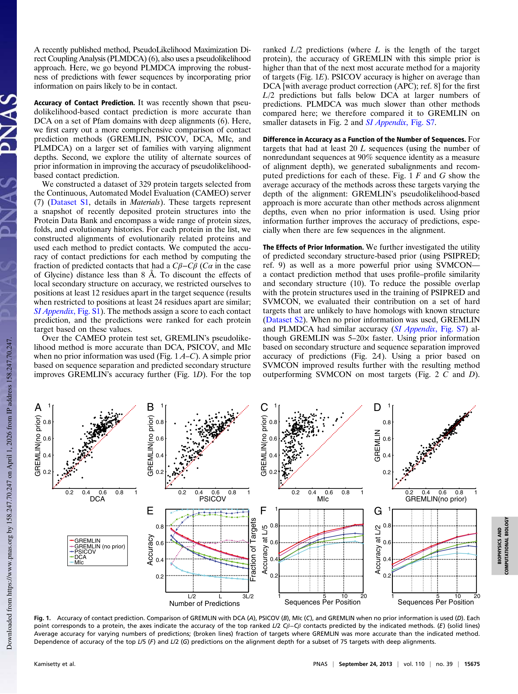
Key observation: The GREMLIN (no prior) vs. GREMLIN (with prior) comparison (panel D) shows points tightly clustered on the diagonal. The prior gives a small bump at shallow depths, but the real gap is between GREMLIN and DCA/PSICOV (panels A–C). The improvement comes from dropping the Gaussian approximation, not from the prior.
Two separable contributions:
- Pseudolikelihood over mean-field — the big win, purely better inference on the same model
- Prior-informed regularization — nice-to-have at shallow depths, not the main story
The Catch-22: When Do Contacts Actually Help?
This is what makes the paper exceptional. They don't just show GREMLIN is better — they rigorously ask when it matters. And they find a catch-22:
- Contact predictions are accurate when the MSA has >5L sequences (L = protein length, at 90% identity filtering)
- But families with that many sequences usually also have a close structural homolog in the PDB — so you can just do comparative modeling
- Contacts are most useful when MSA sequences are more similar to the query than to the closest structural homolog (HHΔ > 0.5)
They categorize all 329 CAMEO targets:
| Category | % | Meaning |
|---|---|---|
| I | 40% | Contact info not useful — can't discriminate native from models |
| II | 29% | Can rank models but can't beat the best comparative model |
| III | 10% | Can actually improve beyond comparative modeling — the sweet spot |
Across all of Pfam: only 422 out of 12,452 families (~3.4%) have both enough sequences for accurate prediction AND no close structural homolog. That's the real target list.
The paper is remarkably honest for a methods paper: it shows the tool is good, then shows that the cases where it actually helps are rare. But those 422 families became the target list for the Baker lab's next landmark: Ovchinnikov et al. 2015, which determined structures of ~600 previously unsolved protein families using GREMLIN contacts + Rosetta.
The Pipeline That Changed Structural Biology
The GREMLIN framework evolved into a pipeline that reshaped the field:
- GREMLIN (2013, this paper): Pseudolikelihood inference of the Potts model, contact prediction
- Ovchinnikov et al. 2015 (eLife): GREMLIN contacts fed into Rosetta → ~600 new protein family structures solved
- trRosetta (2020): Replace hand-crafted Rosetta assembly with a neural network predicting distance/angle distributions from coevolution features
- RoseTTAFold / AlphaFold2 (2021): End-to-end from MSA to structure, with the Evoformer inheriting the two-track decomposition
The prior mechanism in GREMLIN foreshadowed the idea that you could combine coevolutionary signal with other sources of structural information — which is exactly what trRosetta and AlphaFold2 do, just with learned representations instead of hand-crafted priors.
And the conditional probability output P(a at position i | rest) from the fitted Potts model is exactly what protein language models like ESM compute via masked language modeling — but ESM learns it implicitly from raw sequences across all families, while GREMLIN fits it explicitly from a single family's MSA.
Key References Discussed
- Morcos F et al. Direct-coupling analysis of residue coevolution captures native contacts across many protein families. PNAS 108:E1293–E1301, 2011. doi:10.1073/pnas.1111471108 — DCA: mean-field approximation, covariance matrix inversion.
- Jones DT et al. PSICOV: Precise structural contact prediction using sparse inverse covariance estimation. Bioinformatics 28:184–190, 2012. doi:10.1093/bioinformatics/btr638 — Graphical lasso approach with L1 sparsity.
- Ekeberg M et al. Improved contact prediction in proteins: using pseudolikelihoods to infer Potts models. Phys Rev E 87:012707, 2013. doi:10.1103/PhysRevE.87.012707 — PLMDCA: first pseudolikelihood approach, showed superiority over mean-field.
- Ovchinnikov S et al. Large-scale determination of previously unsolved protein structures using evolutionary information. eLife 4:e09248, 2015. doi:10.7554/eLife.09248 — Used GREMLIN contacts + Rosetta to solve ~600 new structures. Direct follow-up to this paper.
- Yang J et al. Improved protein structure prediction using predicted interresidue orientations. PNAS 117:1496–1503, 2020. doi:10.1073/pnas.1914677117 — trRosetta: neural network replacing the GREMLIN → Rosetta pipeline.
- Jumper J et al. Highly accurate protein structure prediction with AlphaFold. Nature 596:583–589, 2021. doi:10.1038/s41586-021-03819-2 — Evoformer architecture inherits the two-track (single-site + pairwise) decomposition from this lineage.